Scientific examples
Complete, runnable programs. Every snippet below was executed against cobranum; the comments show the real output. A few results, visualized:
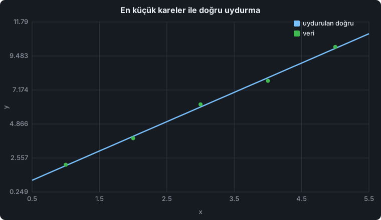
Least-squares line fit (§ regression).
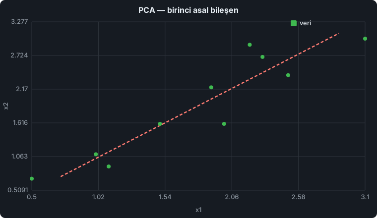
PCA — first principal component.
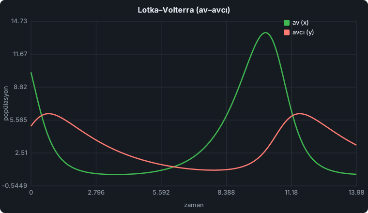
Lotka–Volterra predator–prey (RK4).
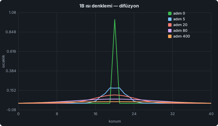
1-D heat equation diffusion.
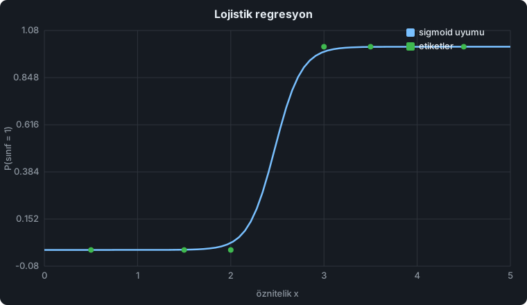
Logistic regression fit.
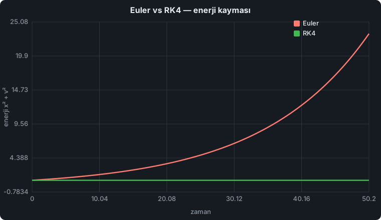
Euler vs RK4 energy drift.
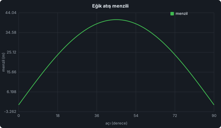
Projectile range vs launch angle.
1 · Descriptive statistics & z-score normalization
Standardize each column of a data matrix to zero mean and unit variance using broadcasting.
import "cobranum.so"
let np = cobranum

let X = np.array([[1, 2, 3], [4, 5, 6], [7, 8, 9]])
let n = np.shape(X)[0]

let mu = np.mul(np.sum(X, 0), 1.0 / n)            # column means (row vector)
let dev = np.sub(X, mu)                            # broadcast subtract
let sd  = np.sqrt(np.mul(np.sum(np.mul(dev, dev), 0), 1.0 / n))
let Z   = np.div(np.sub(X, mu), sd)                # broadcast divide

print(np.to_list(Z))
# => [[-1.2247..., -1.2247..., -1.2247...],
#     [0, 0, 0],
#     [1.2247...,  1.2247...,  1.2247...]]
2 · Linear regression — normal equation
Fit y = Xw in closed form: w = (XᵀX)⁻¹ Xᵀy. The design matrix's first column is the bias term.
let X = np.array([[1, 1], [1, 2], [1, 3], [1, 4]])   # bias + feature
let y = np.array([[2], [3], [4], [5]])               # column vector

let Xt = np.transpose(X)
let w  = np.matmul(np.matmul(np.inv(np.matmul(Xt, X)), Xt), y)

print(np.to_list(w))   # => [[1.0], [1.0]]   (intercept 1, slope 1)
3 · Linear regression — gradient descent
The iterative form, useful when the matrix is large or ill-conditioned. Each step is two matrix products and a scaled subtraction.
let X = np.array([[1, 1], [1, 2], [1, 3], [1, 4]])
let y = np.array([[2], [3], [4], [5]])
let Xt = np.transpose(X)
let n  = np.shape(X)[0]
let lr = 0.05

let w = np.zeros([2, 1])
for step in range(2000)
  let pred = np.matmul(X, w)
  let err  = np.sub(pred, y)
  let grad = np.mul(np.matmul(Xt, err), 1.0 / n)
  w = np.sub(w, np.mul(grad, lr))
end
print(np.to_list(w))   # => [[~1.0], [~1.0]]
4 · Solving linear systems
Solve A x = b with a direct LAPACK solve (LU factorization) — faster and more stable than forming the inverse.
let A = np.array([[3, 2, -1], [2, -2, 4], [-1, 0.5, -1]])
let b = np.array([1, -2, 0])
print(np.to_list(np.solve(A, b)))   # => [1, -2, -2]
5 · Dominant eigenvalue by power iteration
Repeatedly multiply by the matrix and renormalize; the vector converges to the dominant eigenvector and the Rayleigh quotient to its eigenvalue.
let M = np.array([[2, 1], [1, 3]])
let v = np.array([[1], [1]])

for i in range(60)
  let Mv = np.matmul(M, v)
  v = np.div(Mv, np.norm(Mv))        # renormalize (scalar broadcast)
end

let lambda = np.matmul(np.transpose(v), np.matmul(M, v))   # 1x1
print(np.to_list(lambda))   # => [[3.6180...]]   ((5 + sqrt 5) / 2)
6 · Numerical integration (trapezoid rule)
Estimate π from ∫₀¹ 4/(1+x²) dx = π on a fine grid — fully array-native, no loop.
let n = 100000
let x  = np.linspace(0.0, 1.0, n)
let fx = np.div(4.0, np.add(1.0, np.mul(x, x)))      # 4 / (1 + x^2)
let h  = 1.0 / (n - 1)

let area = h * (np.sum(fx) - (np.get(fx, 0) + np.get(fx, n - 1)) / 2.0)
print(area)   # => 3.14159265...
7 · Solving an ODE (Euler integration)
Integrate the harmonic oscillator y' = K y with K = [[0,1],[-1,0]]. After a quarter period the state rotates from (1, 0) to about (0, -1).
let K  = np.array([[0, 1], [-1, 0]])
let dt = 0.01
let state = np.array([[1], [0]])

for i in range(157)                                  # ~ pi/2 in time
  state = np.add(state, np.mul(np.matmul(K, state), dt))
end
print(np.to_list(state))   # => [[~0.0], [~-1.0]]
8 · Markov chain stationary distribution
Iterate a probability row vector through the transition matrix until it stops changing.
let P = np.array([[0.9, 0.1], [0.5, 0.5]])
let v = np.array([[1.0, 0.0]])                       # start in state 0

for i in range(100)
  v = np.matmul(v, P)
end
print(np.to_list(v))   # => [[0.8333..., 0.1666...]]
9 · Polynomial least-squares fit
Fit a quadratic to noisy-looking data by least squares on a Vandermonde matrix. The points lie exactly on y = x² + 1, so the recovered coefficients are [1, 0, 1].
let xs = [0, 1, 2, 3, 4]
let rows = []
for xi in xs
  push(rows, [1.0, xi * 1.0, xi * xi * 1.0])         # [1, x, x^2]
end
let V  = np.array(rows)
let y  = np.reshape(np.array([1, 2, 5, 10, 17]), [5, 1])
let Vt = np.transpose(V)
let coef = np.matmul(np.matmul(np.inv(np.matmul(Vt, V)), Vt), y)

print(np.to_list(coef))   # => [[1.0], [~0.0], [1.0]]   (1 + 0*x + 1*x^2)
10 · Covariance matrix
Center the data and form Cᵀ C / n — the basis of PCA.
let D = np.array([[1, 2], [3, 6], [5, 10], [7, 14]])
let n = np.shape(D)[0]
let mu = np.mul(np.sum(D, 0), 1.0 / n)
let Dc = np.sub(D, mu)                                # center
let cov = np.mul(np.matmul(np.transpose(Dc), Dc), 1.0 / n)
print(np.to_list(cov))   # => [[5, 10], [10, 20]]
11 · Logistic sigmoid & a forward pass
Vectorized σ(z) = 1 / (1 + e⁻ᶻ) over a whole layer, then a one-layer logistic prediction σ(Xw).
let z = np.array([-2, -1, 0, 1, 2])
print(np.to_list(np.div(1.0, np.add(1.0, np.exp(np.neg(z))))))
# => [0.1192..., 0.2689..., 0.5, 0.7310..., 0.8807...]

let X = np.array([[1, 0.5], [1, -1.0], [1, 2.0]])    # samples (with bias)
let w = np.array([[0.2], [0.8]])                     # weights
let probs = np.div(1.0, np.add(1.0, np.exp(np.neg(np.matmul(X, w)))))
print(np.to_list(probs))                             # P(class = 1) per sample
12 · Pairwise vectors & physics — projectile range
Compute the range of a projectile for many launch angles at once: R = v²·sin(2θ)/g, no explicit loop.
let g = 9.81
let v = 20.0
let deg = np.linspace(10.0, 80.0, 8)                 # launch angles
let rad = np.mul(deg, 3.141592653589793 / 180.0)
let R = np.mul(np.sin(np.mul(rad, 2.0)), v * v / g)
print(np.to_list(R))                                 # range per angle (m)
print("max range at index", np.argmax(R))            # ~ 45 degrees